
컨볼루션(convolution)
개요
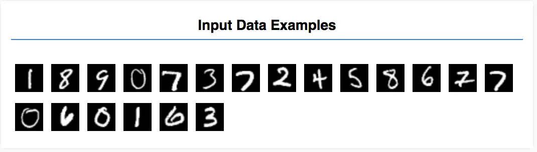
위의 그림과 같은 필기체 이미지를 0 ~ 9 와 같은 숫자로 인식하도록 교육시킨다. (multi-classification)
데이터는 28 * 28px 의 이미지들이며, 1개의 색을 가지는 데이터로 구성되어있다 ([28, 28, 1])
HTML
// index.html
<!DOCTYPE html>
<html>
<head>
<meta charset="utf-8" />
<meta http-equiv="X-UA-Compatible" content="IE=edge" />
<meta name="viewport" content="width=device-width, initial-scale=1.0" />
<title>TensorFlow.js Tutorial</title>
<!-- Import TensorFlow.js -->
<script src="https://cdn.jsdelivr.net/npm/@tensorflow/tfjs@1.0.0/dist/tf.min.js"></script>
<!-- Import tfjs-vis -->
<script src="https://cdn.jsdelivr.net/npm/@tensorflow/tfjs-vis@1.0.2/dist/tfjs-vis.umd.min.js"></script>
<!-- Import the data file -->
<script src="data.js"></script>
<!-- Import the main script file -->
<script src="script.js"></script>
</head>
<body></body>
</html>
HTML
복사
Load Data
// data.js
/**
* @license
* Copyright 2018 Google LLC. All Rights Reserved.
* Licensed under the Apache License, Version 2.0 (the "License");
* you may not use this file except in compliance with the License.
* You may obtain a copy of the License at
*
* http://www.apache.org/licenses/LICENSE-2.0
*
* Unless required by applicable law or agreed to in writing, software
* distributed under the License is distributed on an "AS IS" BASIS,
* WITHOUT WARRANTIES OR CONDITIONS OF ANY KIND, either express or implied.
* See the License for the specific language governing permissions and
* limitations under the License.
* =============================================================================
*/
const IMAGE_SIZE = 784;
const NUM_CLASSES = 10;
const NUM_DATASET_ELEMENTS = 65000;
const TRAIN_TEST_RATIO = 5 / 6;
const NUM_TRAIN_ELEMENTS = Math.floor(TRAIN_TEST_RATIO * NUM_DATASET_ELEMENTS);
const NUM_TEST_ELEMENTS = NUM_DATASET_ELEMENTS - NUM_TRAIN_ELEMENTS;
const MNIST_IMAGES_SPRITE_PATH =
'https://storage.googleapis.com/learnjs-data/model-builder/mnist_images.png';
const MNIST_LABELS_PATH =
'https://storage.googleapis.com/learnjs-data/model-builder/mnist_labels_uint8';
/**
* A class that fetches the sprited MNIST dataset and returns shuffled batches.
*
* NOTE: This will get much easier. For now, we do data fetching and
* manipulation manually.
*/
export class MnistData {
constructor() {
this.shuffledTrainIndex = 0;
this.shuffledTestIndex = 0;
}
async load() {
// Make a request for the MNIST sprited image.
const img = new Image();
const canvas = document.createElement('canvas');
const ctx = canvas.getContext('2d');
const imgRequest = new Promise((resolve, reject) => {
img.crossOrigin = '';
img.onload = () => {
img.width = img.naturalWidth;
img.height = img.naturalHeight;
const datasetBytesBuffer =
new ArrayBuffer(NUM_DATASET_ELEMENTS * IMAGE_SIZE * 4);
const chunkSize = 5000;
canvas.width = img.width;
canvas.height = chunkSize;
for (let i = 0; i < NUM_DATASET_ELEMENTS / chunkSize; i++) {
const datasetBytesView = new Float32Array(
datasetBytesBuffer, i * IMAGE_SIZE * chunkSize * 4,
IMAGE_SIZE * chunkSize);
ctx.drawImage(
img, 0, i * chunkSize, img.width, chunkSize, 0, 0, img.width,
chunkSize);
const imageData = ctx.getImageData(0, 0, canvas.width, canvas.height);
for (let j = 0; j < imageData.data.length / 4; j++) {
// All channels hold an equal value since the image is grayscale, so
// just read the red channel.
datasetBytesView[j] = imageData.data[j * 4] / 255;
}
}
this.datasetImages = new Float32Array(datasetBytesBuffer);
resolve();
};
img.src = MNIST_IMAGES_SPRITE_PATH;
});
const labelsRequest = fetch(MNIST_LABELS_PATH);
const [imgResponse, labelsResponse] =
await Promise.all([imgRequest, labelsRequest]);
this.datasetLabels = new Uint8Array(await labelsResponse.arrayBuffer());
// Create shuffled indices into the train/test set for when we select a
// random dataset element for training / validation.
this.trainIndices = tf.util.createShuffledIndices(NUM_TRAIN_ELEMENTS);
this.testIndices = tf.util.createShuffledIndices(NUM_TEST_ELEMENTS);
// Slice the the images and labels into train and test sets.
this.trainImages =
this.datasetImages.slice(0, IMAGE_SIZE * NUM_TRAIN_ELEMENTS);
this.testImages = this.datasetImages.slice(IMAGE_SIZE * NUM_TRAIN_ELEMENTS);
this.trainLabels =
this.datasetLabels.slice(0, NUM_CLASSES * NUM_TRAIN_ELEMENTS);
this.testLabels =
this.datasetLabels.slice(NUM_CLASSES * NUM_TRAIN_ELEMENTS);
}
nextTrainBatch(batchSize) {
return this.nextBatch(
batchSize, [this.trainImages, this.trainLabels], () => {
this.shuffledTrainIndex =
(this.shuffledTrainIndex + 1) % this.trainIndices.length;
return this.trainIndices[this.shuffledTrainIndex];
});
}
nextTestBatch(batchSize) {
return this.nextBatch(batchSize, [this.testImages, this.testLabels], () => {
this.shuffledTestIndex =
(this.shuffledTestIndex + 1) % this.testIndices.length;
return this.testIndices[this.shuffledTestIndex];
});
}
nextBatch(batchSize, data, index) {
const batchImagesArray = new Float32Array(batchSize * IMAGE_SIZE);
const batchLabelsArray = new Uint8Array(batchSize * NUM_CLASSES);
for (let i = 0; i < batchSize; i++) {
const idx = index();
const image =
data[0].slice(idx * IMAGE_SIZE, idx * IMAGE_SIZE + IMAGE_SIZE);
batchImagesArray.set(image, i * IMAGE_SIZE);
const label =
data[1].slice(idx * NUM_CLASSES, idx * NUM_CLASSES + NUM_CLASSES);
batchLabelsArray.set(label, i * NUM_CLASSES);
}
const xs = tf.tensor2d(batchImagesArray, [batchSize, IMAGE_SIZE]);
const labels = tf.tensor2d(batchLabelsArray, [batchSize, NUM_CLASSES]);
return {xs, labels};
}
}
JavaScript
복사
•
해당 학습에서는 이미지의 digit 을 학습하는 모델을 만들어볼 것
•
MnistData class 에서는 다음의 두 함수가 핵심이다
◦
nextTrainBatch(batchSize): 학습 데이터 셋에서 이미지, 라벨의 랜덤 배치들을 return 한다.
◦
nextTestBatch(batchSize): 테스트 셋에서 이미지, 라벨의 배치들을 return한다
◦
그리고 데이터들을 shuffle 과 normalize 도 실행함.
// script.js
document.addEventListener("DOMContentLoaded", run);
async function run() {
const data = new MnistData();
await data.load();
await showExamples(data);
const model = getModel();
tfvis.show.modelSummary({name: 'Model Architecture'}, model);
await train(model, data);
}
async function showExamples(data) {
// Create a container in the visor
const surface = tfvis
.visor()
.surface({ name: "Input Data Examples", tab: "Input Data" });
// Get the examples
const examples = data.nextTestBatch(20);
const numExamples = examples.xs.shape[0];
// Create a canvas element to render each example
for (let i = 0; i < numExamples; i++) {
const imageTensor = tf.tidy(() => {
// Reshape the image to 28x28 px
return examples.xs
.slice([i, 0], [1, examples.xs.shape[1]])
.reshape([28, 28, 1]);
});
const canvas = document.createElement("canvas");
canvas.width = 28;
canvas.height = 28;
canvas.style = "margin: 4px;";
await tf.browser.toPixels(imageTensor, canvas);
surface.drawArea.appendChild(canvas);
imageTensor.dispose();
}
}
JavaScript
복사
Define Model
function getModel() {
const model = tf.sequential();
const IMAGE_WIDTH = 28;
const IMAGE_HEIGHT = 28;
const IMAGE_CHANNELS = 1;
// In the first layer of our convolutional neural network we have
// to specify the input shape. Then we specify some parameters for
// the convolution operation that takes place in this layer.
model.add(tf.layers.conv2d({
inputShape: [IMAGE_WIDTH, IMAGE_HEIGHT, IMAGE_CHANNELS],
kernelSize: 5,
filters: 8,
strides: 1,
activation: 'relu',
kernelInitializer: 'varianceScaling'
}));
// The MaxPooling layer acts as a sort of downsampling using max values
// in a region instead of averaging.
model.add(tf.layers.maxPooling2d({poolSize: [2, 2], strides: [2, 2]}));
// Repeat another conv2d + maxPooling stack.
// Note that we have more filters in the convolution.
model.add(tf.layers.conv2d({
kernelSize: 5,
filters: 16,
strides: 1,
activation: 'relu',
kernelInitializer: 'varianceScaling'
}));
model.add(tf.layers.maxPooling2d({poolSize: [2, 2], strides: [2, 2]}));
// Now we flatten the output from the 2D filters into a 1D vector to prepare
// it for input into our last layer. This is common practice when feeding
// higher dimensional data to a final classification output layer.
model.add(tf.layers.flatten());
// Our last layer is a dense layer which has 10 output units, one for each
// output class (i.e. 0, 1, 2, 3, 4, 5, 6, 7, 8, 9).
const NUM_OUTPUT_CLASSES = 10;
model.add(tf.layers.dense({
units: NUM_OUTPUT_CLASSES,
kernelInitializer: 'varianceScaling',
activation: 'softmax'
}));
// Choose an optimizer, loss function and accuracy metric,
// then compile and return the model
const optimizer = tf.train.adam();
model.compile({
optimizer: optimizer,
loss: 'categoricalCrossentropy',
metrics: ['accuracy'],
});
return model;
}
JavaScript
복사
•
위에서 dense 대신에 conv2d layer 를 사용했다.
◦
◦
kernalSize 가 5. convolution filter 의 size 가 5x5 를 의미함.
◦
filters 는 kernel 사이즈의 convolution 에서 filer convolution 의 갯수를 의미함.
◦
image classifier 는 dense layer 에서만 만들 수 있지만 convoution layer 는 많은 이미지 작업에서 효과적이라는 사실이 검증이 되었다.
•
flatten
◦
이미지는 고차원 데이터이고, convolution 연산은 주로 데이터의 사이즈를 키우는 경우가 있다. 최종적으로 classifier layer 에 전달하기 전에 하나의 1차원 배열로 만드는 것이 좋다(좋다기 보다는 classification 에 많이 사용된다). dense layer 는 1차원 tensor 만든다.
•
compute
◦
10개의 가능한 class 에 대해서 확률 분포를 계산하기 위해 softmax 활성화와 함께 dense layer 를 사용. 가장 높은 점수를 받은 클래스가 prediction 의 결과가 될 것
◦
1개의 input 에 대해서 10개의 probabilities (class)가 있기 때문에 units(output layer) 를 10으로 설정한다
•
compile
◦
옵티마이저, 손실함수, 매트릭스를 설정해서 컴파일한다.
◦
위의 케이스에서는 categoricalCrossentopy 를 손실함수로 사용한다. (model 의 output 이 확률 분포일 때 사용됨)
◦
categoricalCrossentopy 함수는 마지막 layer 에서 생성된 확률 분포와 실제 label 이 제공한 확률 분포 사이의 오차를 측정한다.
Train the Model
async function train(model, data) {
const metrics = ['loss', 'val_loss', 'acc', 'val_acc'];
const container = {
name: 'Model Training', styles: { height: '1000px' }
};
const fitCallbacks = tfvis.show.fitCallbacks(container, metrics);
const BATCH_SIZE = 512;
const TRAIN_DATA_SIZE = 5500;
const TEST_DATA_SIZE = 1000;
const [trainXs, trainYs] = tf.tidy(() => {
const d = data.nextTrainBatch(TRAIN_DATA_SIZE);
return [
d.xs.reshape([TRAIN_DATA_SIZE, 28, 28, 1]),
d.labels
];
});
const [testXs, testYs] = tf.tidy(() => {
const d = data.nextTestBatch(TEST_DATA_SIZE);
return [
d.xs.reshape([TEST_DATA_SIZE, 28, 28, 1]),
d.labels
];
});
return model.fit(trainXs, trainYs, {
batchSize: BATCH_SIZE,
validationData: [testXs, testYs],
epochs: 10,
shuffle: true,
callbacks: fitCallbacks
});
}
JavaScript
복사
•
prepare data as tensor
◦
용어
컨볼루션(convolution)
수학적으로 간단히 말하면 두 가지 함수가 섞인 것입니다. 머신러닝에서 컨볼루션은 가중치를 학습시키기 위해 컨볼루셔널 필터와 입력 행렬을 혼합합니다.
컨볼루션이 없으면 머신러닝 알고리즘이 큰 텐서의 모든 셀에 있어서 별도의 가중치를 학습해야 합니다. 예를 들어 2,000x2,000 크기의 이미지를 학습하는 머신러닝 알고리즘은 4백만 개의 개별적인 가중치를 찾아야 됩니다. 컨볼루션이 있기 때문에 머신러닝 알고리즘은 컨볼루셔널 필터에 있는 모든 셀의 가중치만 찾아도 되고, 이로 인해 모델 학습에 필요한 메모리가 크게 줄어듭니다. 컨볼루셔널 필터가 적용되는 경우 모든 셀에 같은 필터가 적용되며, 각 셀에 필터가 곱해집니다.
활성화 함수(activation function)
이전 레이어의 모든 입력에 대한 가중 합을 취하고 출력 값(일반적으로 비선형)을 생성하여 다음 레이어로 전달하는 ReLU, 시그모이드 등의 함수입니다.
정류 선형 유닛(ReLU, Rectified Linear Unit)
•
입력이 음수 또는 0이면 출력은 0입니다.
•
입력이 양수이면 출력은 입력과 같습니다.
컨볼루셔널 필터(convolutional filter)
컨볼루셔널 연산에서 사용되는 두 가지 중 하나입니다. 다른 하나는 입력 행렬의 슬라이스입니다. 컨볼루셔널 필터는 입력 행렬과 순위(차원 수)는 동일하지만 모양은 더 작은 행렬입니다. 예를 들어 입력 행렬이 28x28인 경우 컨볼루셔널 필터는 이보다 작은 2차원 행렬이 됩니다.
사진 조작에서 사용되는 컨볼루셔널 필터는 일반적으로 1과 0으로 구성된 일정한 패턴으로 설정됩니다. 머신러닝에서 컨볼루셔널 필터는 일반적으로 난수로 채워지며 네트워크가 이상적인 값을 학습시킵니다.
교차 엔트로피(cross entropy)
다중 클래스 분류 문제로 일반화한 로그 손실입니다. 교차 엔트로피는 두 확률 분포 간의 차이를 계량합니다.